Linear algebra on n-dimensional arrays (ported)
This page is an adaptation of the Linear algebra on n-dimensional arrays tutorial from the NumPy website.
Learner profile
This tutorial is for people who have a basic understanding of linear algebra and arrays in NumPy and want to see how this works in xarray-einstats.
Learning Objectives
After this tutorial, you should be able to:
Understand how to apply some linear algebra operations to DataArrays without using
.valuesor.to_numpy();Understand how axis and shape properties translate to DataArrays and dims.
Content
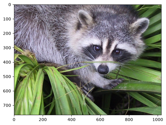
In this tutorial, we will use a matrix decomposition from linear algebra, the Singular Value Decomposition, to generate a compressed approximation of an image. We’ll use the face image from the scipy.datasets module:
from scipy import datasets
import xarray as xr

xr.set_options(display_expand_data=False)

img = xr.DataArray(datasets.face(), dims=["height", "width", "color"], coords={"color": ["R", "G", "B"]})
Downloading file 'face.dat' from 'https://raw.githubusercontent.com/scipy/dataset-face/main/face.dat' to '/home/oriol/.cache/scipy-data'.
Note
If you prefer, you can use your own image as you work through this tutorial. In order to transform your image into a NumPy array that can be manipulated, you can use the imread function from the matplotlib.pyplot submodule. Alternatively, you can use the imageio.imread function from the imageio library. Be aware that if you use your own image, you might need to adapt some steps below.
Now, img is a xarray DataArray, as we can see when using the type function:
type(img)
xarray.core.dataarray.DataArray
We can see the image using matplotlib.pyplot.imshow.
import matplotlib.pyplot as plt

%matplotlib inline
plt.imshow(img)
plt.show()

Dimensions and DataArray properties
In NumPy arrays, dimensions/axis are identified by their positional order, in xarray DataArrays however, dimensions are identified by their name.
We can use .dims to see their names:
img.dims
('height', 'width', 'color')
The output is a tuple with three elements, as we have defined when creating the img variable a few cells above.
However, it is generally not very useful to use .dims for printing. Xarray objects have rich and informative
text and html output:
img
<xarray.DataArray (height: 768, width: 1024, color: 3)> Size: 2MB
121 112 131 138 129 148 153 144 165 155 ... 98 120 156 95 119 155 93 118 154 92
Coordinates:
  * color    (color) <U1 12B 'R' 'G' 'B'
Dimensions without coordinates: height, width
The first line of the output gives the information we got with type, with .dims and more: it also indicates the length of each dimension in addition to their name.
The next lines show a preview of the data, and other fields: coordinates, indexes and attributes.
You might have also noticed that in the first line, the color dimension is in bold face unlike the others.
This is because it has coordinates assigned to index that dimension. Therefore, we can use .sel with the
labels we defined instead of the position to subset the data:
img.sel(color="R")
<xarray.DataArray (height: 768, width: 1024)> Size: 786kB
121 138 153 155 155 158 159 156 147 137 ... 113 116 117 120 121 121 120 119 118
Coordinates:
    color    <U1 4B 'R'
Dimensions without coordinates: height, widthFrom the output above, we can see that every value in red color channel of img is an integer value between 0 and 255, representing the level of red in each corresponding image pixel (keep in mind that this might be different if you
use your own image instead of scipy.datasets.face).
Note the data subset now has two dimensions only: height and width of lengths 768 and 1024 respectively.
Since we are going to perform linear algebra operations on this data, it might be more interesting to have real numbers between 0 and 1 in each entry of the matrices to represent the RGB values. We can do that by setting
img_array = img / 255
This operation, dividing an array by a scalar, works because of NumPy’s and xarray broadcasting. (Note that in real-world applications, it would be better to use, for example, the img_as_float utility function from scikit-image).
You can check that the above works by doing some tests; for example, inquiring about maximum and minimum values for this array:
img_array.max(), img_array.min()
(<xarray.DataArray ()> Size: 8B
 1.0,
 <xarray.DataArray ()> Size: 8B
 0.0)
or checking the type of data in the array:
img_array.dtype
dtype('float64')
Operations on an axis
It is possible to use methods from linear algebra to approximate an existing set of data. Here, we will use the SVD (Singular Value Decomposition) to try to rebuild an image that uses less singular value information than the original one, while still retaining some of its features.
To proceed, import the linear algebra submodule from xarray-einstats:
from xarray_einstats import linalg
In order to extract information from a given matrix, we can use the SVD to obtain 3 arrays which can be multiplied to obtain the original matrix. From the theory of linear algebra, given a matrix \(A\), the following product can be computed:
where \(U\) and \(V^T\) are square and \(\Sigma\) is the same size as \(A\). \(\Sigma\) is a diagonal matrix and contains the singular values of \(A\), organized from largest to smallest. These values are always non-negative and can be used as an indicator of the “importance” of some features represented by the matrix \(A\).
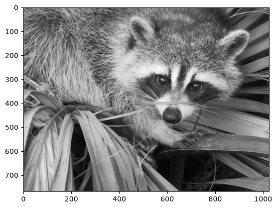
Let’s see how this works in practice with just one matrix first. Note that according to colorimetry, it is possible to obtain a fairly reasonable grayscale version of our color image if we apply the formula
where \(Y\) is the array representing the grayscale image, and \(R\), \(G\) and \(B\) are the red, green and blue channel arrays we had originally. Notice we can use a dot product for this:
color_coefs = xr.DataArray([0.2126, 0.7152, 0.0722], dims=["color"], coords={"color": ["R", "G", "B"]})
img_gray = img_array.dot(color_coefs)
Now, img_gray has shape
img_gray
<xarray.DataArray (height: 768, width: 1024)> Size: 6MB
0.4521 0.5188 0.5782 0.586 0.586 0.5955 ... 0.5667 0.5662 0.5645 0.5603 0.5564
Dimensions without coordinates: height, width
To see if this makes sense in our image, we should use a colormap from matplotlib corresponding to the color we wish to see in out image (otherwise, matplotlib will default to a colormap that does not correspond to the real data).
In our case, we are approximating the grayscale portion of the image, so we will use the colormap gray:
plt.imshow(img_gray, cmap="gray");
Now, applying the linalg.svd function to this matrix, we obtain the following decomposition:
U, s, Vt = img_gray.linalg.svd(dims=["height", "width"])
Attention
If you are using your own image, this command might take a while to run, depending on the size of your image and your hardware. Don’t worry, this is normal! The SVD can be a pretty intensive computation.
Let’s check that this is what we expected:
U
<xarray.DataArray (height: 768, height2: 768)> Size: 5MB
0.03181 0.01899 0.01773 0.00738 0.01887 ... 0.03089 0.005258 0.0146 0.004079
Dimensions without coordinates: height, height2
s
<xarray.DataArray (height: 768)> Size: 6kB
410.4 85.56 63.61 45.85 41.97 38.26 ... 0.01117 0.01085 0.01079 0.01032 0.009925
Dimensions without coordinates: height
Vt
<xarray.DataArray (width: 1024, width2: 1024)> Size: 8MB
0.03587 0.03582 0.03581 0.03574 0.03553 ... 0.03706 0.0731 -0.2073 0.1374
Dimensions without coordinates: width, width2
Note that s has a particular shape: it has only one dimension. This means that some linear algebra functions that expect 2d arrays might not work. For example, from the theory, one might expect s and Vt to be
compatible for multiplication. However, this is not true as s does not have a second axis, and we don’t want to execute a dot product as that would multiply the elements in s for whole columns instead of a matrix multiplication.
This happens because having a one-dimensional array for s, in this case, is much more economic in practice than building a diagonal matrix with the same data. To reconstruct the original matrix, we can rebuild the diagonal matrix \(\Sigma\) with the elements of s in its diagonal and with the appropriate dimensions for multiplying: in our case, \(\Sigma\) should have height, width dimensions. In order to add the singular values to the diagonal of Sigma, we will manually create the indexes and use .loc:
import numpy as np

Sigma = xr.zeros_like(img_gray)
idx = xr.DataArray(np.arange(min(Sigma.shape)), dims="pointwise_sel")
Sigma.loc[{"width": idx, "height": idx}] = s.rename(height="pointwise_sel")
Sigma
<xarray.DataArray (height: 768, width: 1024)> Size: 6MB
410.4 0.0 0.0 0.0 0.0 0.0 0.0 0.0 0.0 ... 0.0 0.0 0.0 0.0 0.0 0.0 0.0 0.0 0.0
Dimensions without coordinates: height, width
Now, we want to check if the reconstructed U @ Sigma @ Vt is close to the original img_gray matrix.
Approximation
The linalg module includes a linalg.norm function, which computes the norm of a vector or matrix represented in a NumPy array. For example, from the SVD explanation above, we would expect the norm of the difference between img_gray and the reconstructed SVD product to be small. As expected, you should see something like
approx = linalg.matmul(
    linalg.matmul(U, Sigma, dims=[["height", "height2"], ["height", "width"]]),
    Vt,
    dims=["height", "width", "width2"],
).rename(width2="width")
linalg.norm(img_gray - approx, dims=("height", "width"))
<xarray.DataArray ()> Size: 8B
1.428e-12
(The actual result of this operation might be different depending on your architecture and linear algebra setup. Regardless, you should see a small number.)
We could also have used the numpy.allclose function to make sure the reconstructed product is, in fact, close to our original matrix (the difference between the two arrays is small):
np.allclose(img_gray, approx)
True
To see if an approximation is reasonable, we can check the values in s:
plt.plot(s)
plt.show()
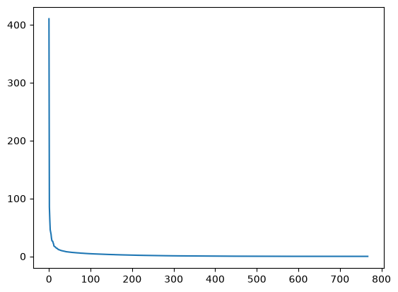
In the graph, we can see that although we have 768 singular values in s, most of those (after the 150th entry or so) are pretty small. So it might make sense to use only the information related to the first (say, 50) singular values to build a more economical approximation to our image.
The idea is to consider all but the first k singular values in Sigma (which are the same as in s) as zeros, keeping U and Vt intact, and computing the product of these matrices as the approximation.
For example, if we choose
k = 10
Sigma.sel(width=slice(0, k))
<xarray.DataArray (height: 768, width: 10)> Size: 61kB
410.4 0.0 0.0 0.0 0.0 0.0 0.0 0.0 0.0 ... 0.0 0.0 0.0 0.0 0.0 0.0 0.0 0.0 0.0
Dimensions without coordinates: height, width
Vt.sel(width=slice(0, k))
<xarray.DataArray (width: 10, width2: 1024)> Size: 82kB
0.03587 0.03582 0.03581 0.03574 0.03553 ... -0.07889 -0.07779 -0.07644 -0.07542
Dimensions without coordinates: width, width2
we can build the approximation by doing
approx = linalg.matmul(
    linalg.matmul(U, Sigma.sel(width=slice(0, k)), dims=[["height", "height2"], ["height", "width"]]),
    Vt.sel(width=slice(0, k)),
    dims=["height", "width", "width2"],
).rename(width2="width")
Note that we had to use only the first k rows of Vt, since all other rows would be multiplied by the zeros corresponding to the singular values we eliminated from this approximation.
plt.imshow(approx, cmap="gray")
plt.show()
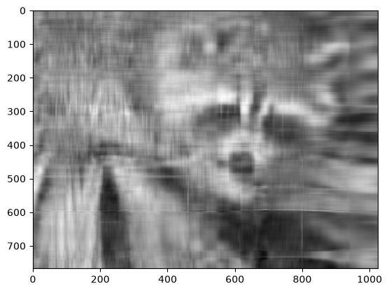
Now, you can go ahead and repeat this experiment with other values of k, and each of your experiments should give you a slightly better (or worse) image depending on the value you choose.
Applying to all colors
Now we want to do the same kind of operation, but to all three colors. Our first instinct might be to repeat the same operation we did above to each color matrix individually. However, xarray-einstats will take care of all this for us (using NumPy’s and xarray’s broadcasting under the hood).
Unlike with raw NumPy where we need to be careful to place the dimensions we want to operate on in the first or last position, with xarray-einstats we indicate the dimensions we want to operate on using the dims argument.
That was quite an overkill so far as the inputs where 2d, yet we still specified which dimensions we wanted to operate on. But the good news come now, nearly everything we have done so far works just the same if we include the color channel too, with no changes, no transposing, no indicating we now have more dimensions… we were operating on the height and width dimensions, so xarray-einstats will do so whether they are the only dimensions or the 3rd and 7th out of a total of 9 dimensions.
U, s, Vt = img_array.linalg.svd(dims=["height", "width"])
Finally, to obtain the full approximated image, we need to reassemble these matrices into the approximation.
Products with n-dimensional arrays
Here is the only modified piece of code: the creation of the Sigma matrix.
# modified code
Sigma = xr.zeros_like(img_array)
min_len = min(len(Sigma["height"]), len(Sigma["width"]))
idx = xr.DataArray(np.arange(min_len), dims="height")

Sigma.loc[{"height": idx, "width": idx}] = s.transpose()  # the transpose is a workaround due to https://github.com/pydata/xarray/issues/7030
Now, if we wish to rebuild the full SVD (with no approximation), we can do
reconstructed = linalg.matmul(
    linalg.matmul(U, Sigma, dims=[["height", "height2"], ["height", "width"]]),
    Vt,
    dims=["height", "width", "width2"],
).rename(width2="width")
reconstructed
<xarray.DataArray (color: 3, height: 768, width: 1024)> Size: 19MB
0.4745 0.5412 0.6 0.6078 0.6078 0.6196 ... 0.3922 0.3843 0.3725 0.3647 0.3608
Coordinates:
  * color    (color) <U1 12B 'R' 'G' 'B'
Dimensions without coordinates: height, width
The reconstructed image should be indistinguishable from the original one, except for differences due to floating point errors from the reconstruction. Recall that our original image consisted of floating point values in the range [0., 1.]. The accumulation of floating point error from the reconstruction can result in values slightly outside this original range:
reconstructed.min(), reconstructed.max()
(<xarray.DataArray ()> Size: 8B
 -7.736e-15,
 <xarray.DataArray ()> Size: 8B
 1.0)
Since imshow expects values in the range, we can use clip to excise the floating point error:
reconstructed = np.clip(reconstructed, 0, 1)
plt.imshow(reconstructed.transpose(..., "color"));
In fact, imshow peforms this clipping under-the-hood, so if you skip the first line in the previous code cell, you might see a warning message saying "Clipping input data to the valid range for imshow with RGB data ([0..1] for floats or [0..255] for integers)."
Now, to do the approximation, we must choose only the first k singular values for each color channel. This can be done using the following syntax:
approx = linalg.matmul(
    linalg.matmul(U, Sigma.sel(width=slice(0, k)), dims=[["height", "height2"], ["height", "width"]]),
    Vt.sel(width=slice(0, k)),
    dims=["height", "width", "width2"],
).rename(width2="width")
You can see that we have selected only the first k components of the last axis for Sigma (this means that we have used only the first k columns of each of the three matrices in the stack), and that we have selected only the first k components in the second-to-last axis of Vt (this means we have selected only the first k rows from every matrix in the stack Vt and all columns). If you are unfamiliar with the ellipsis syntax, it is a
placeholder for other axes. For more details, see the documentation on Indexing.
Now,
approx
<xarray.DataArray (color: 3, height: 768, width: 1024)> Size: 19MB
0.4745 0.4822 0.4893 0.492 0.4967 0.5061 ... 0.2838 0.2866 0.2899 0.2925 0.2938
Coordinates:
  * color    (color) <U1 12B 'R' 'G' 'B'
Dimensions without coordinates: height, width
which is not the right shape for showing the image. We need to place the color dimension as last to be able to plot with matplotlib:
approx = np.clip(approx, 0, 1)
plt.imshow(approx.transpose(..., "color"));
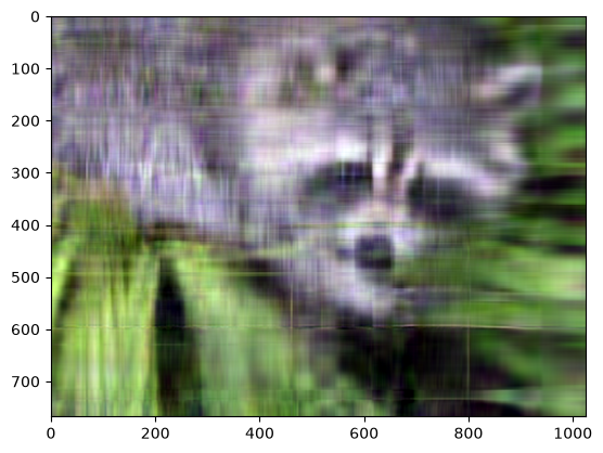
Even though the image is not as sharp, using a small number of k singular values (compared to the original set of 768 values), we can recover many of the distinguishing features from this image.
Final words
Of course, this is not the best method to approximate an image. However, there is, in fact, a result in linear algebra that says that the approximation we built above is the best we can get to the original matrix in terms of the norm of the difference. For more information, see G. H. Golub and C. F. Van Loan, Matrix Computations, Baltimore, MD, Johns Hopkins University Press, 1985.
Further reading
%load_ext watermark
%watermark -n -u -v -iv -w
Last updated: Mon, 20 Jul 2026

Python implementation: CPython
Python version       : 3.14.6
IPython version      : 9.15.0

matplotlib     : 3.11.1
numpy          : 2.5.1
scipy          : 1.18.0
xarray         : 2026.7.0
xarray_einstats: 0.11.0

Watermark: 2.6.0