Intro to the stats module#
from scipy import stats
import numpy as np
from xarray_einstats.stats import XrContinuousRV, rankdata, hmean, skew, median_abs_deviation
from xarray_einstats.tutorial import generate_mcmc_like_dataset
ds = generate_mcmc_like_dataset(11)
Probability distributions#
Initialization#
norm = XrContinuousRV(stats.norm, ds["mu"], ds["sigma"])
Using its methods#
Once initialized, you can use its methods exactly as you’d use them with scipy distributions. The only two differences are
They now take scalars or DataArrays as inputs, arrays are only accepted as the arguments on which to evaluate the methods (in scipy docs they are represented by
x,korqdepending on the method)sizebehaves differently in thervsmethod. This ensures that you don’t need to care about any broadcasting or alignment of arrays,xarray_einstatsdoes this for you.
You can generate 10 random draws from the initialized distribution. Here, unlike what would happen with scipy, the output won’t have shape 10, but instead will have shape 10, *broadcasted_input_shape. xarray generates the broadcasted_input_shape and size is independent from it so you can relax and not care about broadcasting.
norm.rvs(size=(10))
<xarray.DataArray (rv_dim0: 10, chain: 4, draw: 10, team: 6)>
-0.02342 0.4384 1.526 0.2427 -0.3344 ... 0.04699 -0.5903 -0.2142 0.6762 1.661
Coordinates:
  * team     (team) <U1 'a' 'b' 'c' 'd' 'e' 'f'
  * chain    (chain) int64 0 1 2 3
  * draw     (draw) int64 0 1 2 3 4 5 6 7 8 9
Dimensions without coordinates: rv_dim0
If the dimension names are not provided, xarray_einstats assings rv_dim# as dimension name as many times as necessary. To define the names manually you can use the dims argument:
norm.rvs(size=(5, 3), dims=["subject", "batch"])
<xarray.DataArray (subject: 5, batch: 3, chain: 4, draw: 10, team: 6)>
0.4488 0.4036 0.3949 0.708 0.7141 3.845 ... 0.1895 -0.03576 0.3021 0.5014 1.839
Coordinates:
  * team     (team) <U1 'a' 'b' 'c' 'd' 'e' 'f'
  * chain    (chain) int64 0 1 2 3
  * draw     (draw) int64 0 1 2 3 4 5 6 7 8 9
Dimensions without coordinates: subject, batch
The behaviour for other methods is similar:
norm.logcdf(ds["x_plot"])
<xarray.DataArray (plot_dim: 20, chain: 4, draw: 10, team: 6)>
-1.318 -2.617 -6.71 -0.7968 ... -1.248e-263 -7.905e-247 -1.896e-242 -1.636e-170
Coordinates:
  * chain    (chain) int64 0 1 2 3
  * draw     (draw) int64 0 1 2 3 4 5 6 7 8 9
  * team     (team) <U1 'a' 'b' 'c' 'd' 'e' 'f'
Dimensions without coordinates: plot_dim
For convenience, you can also use array_like input which is converted to a DataArray under the hood. In such cases, the dimension name is quantile for ppf and isf, point otherwise. In both cases, the values passed as input are preserved as coordinate values.
norm.ppf([.25, .5, .75])
<xarray.DataArray (quantile: 3, chain: 4, draw: 10, team: 6)>
-0.02018 0.2885 0.8726 -0.204 -0.1332 ... 0.2786 0.2264 0.5523 0.6391 2.198
Coordinates:
  * quantile  (quantile) float64 0.25 0.5 0.75
  * chain     (chain) int64 0 1 2 3
  * draw      (draw) int64 0 1 2 3 4 5 6 7 8 9
  * team      (team) <U1 'a' 'b' 'c' 'd' 'e' 'f'
pdf = norm.pdf(np.linspace(-5, 5))
pdf
<xarray.DataArray (point: 50, chain: 4, draw: 10, team: 6)>
5.321e-44 2.898e-49 4.753e-60 5.206e-41 ... 3.563e-57 4.449e-55 3.664e-24
Coordinates:
  * point    (point) float64 -5.0 -4.796 -4.592 -4.388 ... 4.388 4.592 4.796 5.0
  * chain    (chain) int64 0 1 2 3
  * draw     (draw) int64 0 1 2 3 4 5 6 7 8 9
  * team     (team) <U1 'a' 'b' 'c' 'd' 'e' 'f'
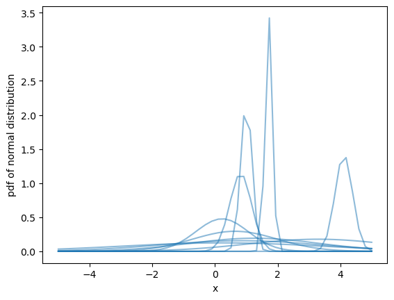
Plot a subset of the pdf we just calculated with matplotlib.
import matplotlib.pyplot as plt
plt.rcParams["figure.facecolor"] = "white"

fig, ax = plt.subplots()
ax.plot(pdf.point, pdf.sel(team="d", chain=2), color="C0", alpha=.5)
ax.set(xlabel="x", ylabel="pdf of normal distribution", );
Other functions#
The rest of the functions in the module have a very similar API to their scipy counterparts, the only differences are:
They take
dimsinstead ofaxis. Moreover,dimscan bestror a sequence ofstrinstead of a single integer only as supported byaxis.Arguments that take array_like as values take
DataArrayinputs instead. For example thescaleargument inmedian_abs_deviationThey accept extra arbitrary kwargs, that are passed to
xarray.apply_ufunc.
Here are some examples of using functions in the stats module of xarray_einstats with dims argument instead of axis.
hmean(ds["mu"], dims="team")
<xarray.DataArray 'mu' (chain: 4, draw: 10)>
0.1588 0.2123 0.5543 0.7826 0.1913 0.6035 ... 0.1269 0.712 0.3044 0.1936 0.1223
Coordinates:
  * chain    (chain) int64 0 1 2 3
  * draw     (draw) int64 0 1 2 3 4 5 6 7 8 9
rankdata(ds["score"], dims=("chain", "draw"), method="min")
<__array_function__ internals>:200: RuntimeWarning: invalid value encountered in cast
<xarray.DataArray 'score' (match: 12, chain: 4, draw: 10)>
14 14 14 14 14 31 14 1 31 14 31 1 14 1 ... 15 15 15 15 15 1 34 15 15 1 34 34 34
Dimensions without coordinates: match, chain, draw
Important
The statistical summaries and other statistical functions can take both DataArray and Dataset. Methods in probability functions and functions in linear algebra module
are tested only on DataArrays.
When using Dataset inputs, you must make sure that all the dimensions in dims are
present in all the DataArrays within the Dataset.
skew(ds[["score", "mu", "sigma"]], dims=("chain", "draw"))
<xarray.Dataset>
Dimensions:  (match: 12, team: 6)
Coordinates:
  * team     (team) <U1 'a' 'b' 'c' 'd' 'e' 'f'
Dimensions without coordinates: match
Data variables:
    score    (match) float64 1.466 0.2149 0.6788 1.361 ... 1.099 1.156 1.265
    mu       (team) float64 0.8152 1.84 2.102 1.806 1.091 0.9678
sigma float64 1.314median_abs_deviation(ds)
<xarray.Dataset>
Dimensions:  ()
Data variables:
    x_plot   float64 2.632
    mu       float64 0.4878
    sigma    float64 0.39
score float64 1.0%load_ext watermark
%watermark -n -u -v -iv -w -p xarray_einstats,xarray
Last updated: Tue Jul 11 2023

Python implementation: CPython
Python version       : 3.10.12
IPython version      : 8.14.0

xarray_einstats: 0.6.0
xarray         : 2023.6.0

scipy     : 1.11.1
numpy     : 1.24.4
matplotlib: 3.7.1

Watermark: 2.4.3