Einops tutorial (ported)

This tutorial is a port using xarray-einstats of the einops basics tutorial

Einops meets xarray!

We don’t write

y = x.transpose(0, 2, 3, 1)

nor we write the more comprehensible alternative

y = rearrange(x, 'b c h w -> b h w c')

we write comprehensible code and use labeled arrays

y_da = rearrange(x_da, 'batch height width channel')
# or, also equivalent
y_da = x_da.einops.rearrange('batch height width channel')

x_da is a xarray.DataArray whose dimensions are already labeled, thus, we can skip the left side that defines the names of the dimensions.

xarray-einstats wraps einops functions to extend them to work on xarray objects.

What’s in this tutorial?

• fundamentals: reordering, composition and decomposition of axes

• operations: rearrange, reduce, repeat

• how much you can do with a single operation!

Preparations

# Examples are given for numpy. This code also setups ipython/jupyter
# so that numpy arrays in the output are displayed as images
import numpy
import xarray
from xarray_einstats.tutorial import display_np_arrays_as_images
display_np_arrays_as_images()

Note

This cell above configures jupyter to display numpy arrays as images, which is a great visual help to understand the operations performed by einops. To take advantage of this we use .values. In some specific cases, we also omit it in order to show the values of the dimensions of the DataArray. If you are running this yourself we encourage you to try both views

Load a batch of images to play with

Download the data for local use

The images are stored as a zarr store in the xarray-einstats repo. You can download it directly from your browser using https://download-directory.github.io/ and pasting https://github.com/arviz-devs/xarray-einstats/tree/main/docs/source/tutorials/einops-image.zarr there. Then move the file if necessary, uncompress and rename it so you can load it with open_zarr as shown below.

ds = xarray.open_zarr("einops-image.zarr").load()
ims = ds["ims"]
# There are 6 images of shape 96x96 with 3 color channels packed into the ims DataArray
ds

<xarray.Dataset>
Dimensions:  (batch: 6, height: 96, width: 96, channel: 3)
Dimensions without coordinates: batch, height, width, channel
Data variables:
    ims      (batch, height, width, channel) float64 1.0 0.902 ... 1.0 0.8039

xarray.Dataset

• Dimensions:
  • batch: 6
  • height: 96
  • width: 96
  • channel: 3
• Coordinates: (0)
• Data variables: (1)
  • ims
    (batch, height, width, channel)
    float64
    1.0 0.902 0.902 ... 1.0 1.0 0.8039

    array([[[[1.        , 0.90196078, 0.90196078],
             [1.        , 0.90196078, 0.90196078],
             [1.        , 0.90196078, 0.90196078],
             ...,
             [1.        , 0.90196078, 0.90196078],
             [1.        , 0.90196078, 0.90196078],
             [1.        , 0.90196078, 0.90196078]],
    
            [[1.        , 0.90196078, 0.90196078],
             [1.        , 0.90196078, 0.90196078],
             [1.        , 0.90196078, 0.90196078],
             ...,
             [1.        , 0.90196078, 0.90196078],
             [1.        , 0.90196078, 0.90196078],
             [1.        , 0.90196078, 0.90196078]],
    
            [[1.        , 0.90196078, 0.90196078],
             [1.        , 0.90196078, 0.90196078],
             [1.        , 0.90196078, 0.90196078],
             ...,
    ...
             ...,
             [1.        , 1.        , 0.80392157],
             [1.        , 1.        , 0.80392157],
             [1.        , 1.        , 0.80392157]],
    
            [[1.        , 1.        , 0.80392157],
             [1.        , 1.        , 0.80392157],
             [1.        , 1.        , 0.80392157],
             ...,
             [1.        , 1.        , 0.80392157],
             [1.        , 1.        , 0.80392157],
             [1.        , 1.        , 0.80392157]],
    
            [[1.        , 1.        , 0.80392157],
             [1.        , 1.        , 0.80392157],
             [1.        , 1.        , 0.80392157],
             ...,
             [1.        , 1.        , 0.80392157],
             [1.        , 1.        , 0.80392157],
             [1.        , 1.        , 0.80392157]]]])

• Indexes: (0)
• Attributes: (0)

display the first image (whole 4d tensor can’t be rendered)

ims.sel(batch=0).values

second image in a batch

ims.sel(batch=1).values

we’ll use three operations

from xarray_einstats.einops import rearrange, reduce #, repeat

rearrange, as its name suggests, rearranges elements.

Below we swapped height and width. This can be seen as transposing the first two dimensions, but in xarray, by design, the order of the dimensions should not matter, and that exact code below should (and will work) if the input object has the same dimension names but different order (in which case the operation might be transposing 1st and 3rd dims) or doing nothing. Having said that, rearranging is still a valuable operation on xarray objects, especially if done right before accessing the underlying numpy or dask array.

By rearranging, we are enforcing the width, height, channel order.

ims.sel(batch=0).einops.rearrange('width height channel').values

Composition of axes

transposition is very common and useful, but let’s move to other capabilities provided by einops

einops allows seamlessly composing batch and height to a new height dimension, something that tends to be tricky in xarray once we move from a standard stack.

We just rendered all images by collapsing to 3d tensor!

da = rearrange(ims, '(batch height) width channel')
da.values

but wait, dimensions must be named in xarray, so what happened with this stacked dimension we have just created?

xarray_einstats assigns it a dimension name based on the names of the parent dimensions:

da.dims

('batch-height', 'width', 'channel')

we can also compose a new dimension of batch and width. And now we will name it manually (strongly recommended over relying on the automatic names)

ims.einops.rearrange('(batch width)=batched_widths channel').values

note that here we have skipped the height dimension not only from the input but also from the output expression. xarray_einstats follows xarray convention of adding the new or modified (aka present in the output expression) dimensions at the end.

As dimensions are already named, we can skip dimensions not only from the input as we have been doing but also from the output if we don’t mind the new dimensions being moved to the right of the omitted ones.

Resulting dimensions are computed very simply. The length of newly composed axis is a product of components: [6, 96, 96, 3] -> [96, (6 * 96), 3]

rearrange(ims, '(batch width) channel').shape

(96, 576, 3)

We can compose more than two axes. Let’s flatten 4d array into 1d, resulting array has as many elements as the original

rearrange(ims, '(batch height width channel)').shape

(165888,)

Note

Everything we have done so far could have been done with transpose or with stack, so choosing between those methods or einops is a matter of personal choice. We’d recommend you stick with the original xarray methods, especially if working with dask arrays, their defaults will be much more convenient than the lack of automatic dask handling in xarray_einstats.

The rearrangements below this point however can’t be reproduced by a single xarray method.

Decomposition of axis

Decomposition is the inverse process, we represent an axis as a combination of new axes.

There will always be several decompositions possible, so we specify b1=2 to decompose batch to two dimensions b1 and b2 of lengths 2 and 3 respectively.

In addition, we also need to specify the name of the dimension we want to decompose.

ims.einops.rearrange('(b1 b2)=batch -> b1 b2 height width channel ', b1=2).shape

(2, 3, 96, 96, 3)

Finally, combine composition and decomposition:

da = rearrange(ims, '(b1 b2)=batch -> (b1 height) (b2 width) channel ', b1=2)
da.values

Again, we skip naming the output dimensions so they are named by xarray_einstats

da.dims

('b1-height', 'b2-width', 'channel')

Slightly different composition: b1 is merged with width, b2 with height

… so letters are ordered by w then by h

rearrange(ims, '(b1 b2)=batch -> (b2 height) (b1 width) channel ', b1=2).values

Wove part of width dimension to height. We should call this width-to-height as image width shrunk by 2 and height doubled.

but all pixels are the same!

Can you write reverse operation (height-to-width)?

rearrange(ims, '(w1 w2)=width -> (height w2) (batch w1) channel', w2=2).values

Order of axes matters

Compare with the next two examples

rearrange(ims, '(batch width) channel').values

rearrange(ims, '(width batch) channel').values

The order of axes in the composition is different.

The rule is just as for digits in the number: the leftmost digit is the most significant, while neighboring numbers differ in the rightmost axis. You can also think of this as lexicographic sort

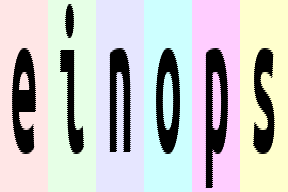
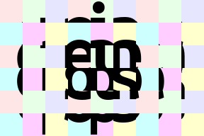
And what if b1 and b2 are reordered before composing to width?

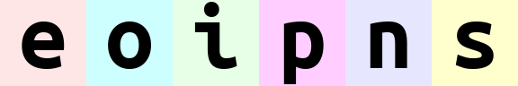
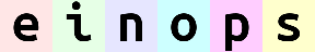
rearrange(ims, '(b1 b2)=batch -> (b1 b2 width) channel ', b1=2).values # produces 'einops'
rearrange(ims, '(b1 b2)=batch -> (b2 b1 width) channel ', b1=2).values # produces 'eoipns'

Meet reduce

From einops documentation:

In einops-land you don’t need to guess what happened

x.mean(-1)

Because you write what the operation does

reduce(x, 'b h w c -> b h w', 'mean')

if an axis is not present in the output — you guessed it — that axis is reduced.

using xarray objects, you already don’t have to guess what happened. Much like with rearrange, the first examples (three in this case) using reduce can be reproduced with a single xarray method. See the operation above with pure xarray and with reduce:

da.mean("channel")
reduce(x, "batch width height", "mean")

However, again much like with rearrange, reduce also opens the door to many other operations that go beyond what single xarray methods can do. These cases are worth making reduce work, and once it’s working the simple operations are possible automatically.

If you prefer thinking in terms of the dimensions that are kept instead of the ones that are reduced, using reduce can be more convenient even for simple operations.

# average over batch
ims.einops.reduce('height width channel', 'mean').values

# the previous is identical to familiar:
ims.values.mean(axis=0)
# but is so much more readable

# Example of reducing of several axes 
# besides mean, there are also min, max, sum, prod
reduce(ims, 'height width', 'min').values

# this is mean-pooling with 2x2 kernel
# image is split into 2x2 patches, each patch is averaged
reduce(ims, '(h h2)=height (w w2)=width -> h (batch w) channel', 'mean', h2=2, w2=2).values

# max-pooling is similar
# result is not as smooth as for mean-pooling
ims.einops.reduce('(h h2)=height (w w2)=width -> h (batch w) channel', 'max', h2=2, w2=2).values

# yet another example. Can you compute result shape?
reduce(ims, '(b1 b2)=batch -> (b2 height) (b1 width)', 'mean', b1=2).values

We skip the section about numpy-like stacking and concatenating because they aren’t relevant to xarray objects.

We have also reimagined the next section. We are working with xarray objects so adding new axis of length 1 to ensure broadcastability is not relevant either. We have therefore modified the section to a showcase of xarray automatic broadcasting and alignment.

Broadcasting and alignment

As we are using xarray objects, we can directly operate between original and reduced inputs without the need for adding new dimensions, be it with [np.newaxis, :] or with 1 and () placeholders in einops expressions. See for yourself:

# compute max in each image individually, then show a difference 
x = reduce(ims, 'batch channel', 'max') - ims
rearrange(x, '(batch width) channel').values

Repeating elements

coming soon, for now jump to Fancy examples in random order

Third operation we introduce is repeat

# repeat along a new axis. New axis can be placed anywhere
repeat(ims[0], 'h w c -> h new_axis w c', new_axis=5).shape

# shortcut
repeat(ims[0], 'h w c -> h 5 w c').shape

# repeat along w (existing axis)
repeat(ims[0], 'h w c -> h (repeat w) c', repeat=3)

# repeat along two existing axes
repeat(ims[0], 'h w c -> (2 h) (2 w) c')

# order of axes matters as usual - you can repeat each element (pixel) 3 times 
# by changing order in parenthesis
repeat(ims[0], 'h w c -> h (w repeat) c', repeat=3)

Note: repeat operation covers functionality identical to numpy.repeat, numpy.tile and actually more than that.

Reduce ⇆ repeat

reduce and repeat are like opposite of each other: first one reduces amount of elements, second one increases.

In the following example each image is repeated first, then we reduce over new axis to get back original tensor. Notice that operation patterns are “reverse” of each other

repeated = repeat(ims, 'b h w c -> b h new_axis w c', new_axis=2)
reduced = reduce(repeated, 'b h new_axis w c -> b h w c', 'min')
assert numpy.array_equal(ims, reduced)

Fancy examples in random order

(a.k.a. mad designer gallery)

# interweaving pixels of different pictures
# all letters are observable
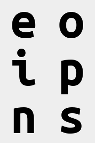
rearrange(ims, '(b1 b2)=batch -> (height b1) (width b2) channel ', b1=2).values

# interweaving along vertical for couples of images
ims.einops.rearrange('(b1 b2)=batch -> (height b1) (b2 width) channel', b1=2).values

# interweaving lines for couples of images
# exercise: achieve the same result without einops in your favourite framework
reduce(ims, '(b1 b2)=batch -> height (b2 width) channel', 'max', b1=2).values

# color can be also composed into dimension
# ... while image is downsampled
reduce(ims, '(h h2)=height (w w2)=width -> (channel h) (batch w)', 'mean', h2=2, w2=2).values

# disproportionate resize
reduce(ims, '(h h4)=height (w w3)=width -> h (batch w)', 'mean', h4=4, w3=3).values

# spilt each image in two halves, compute mean of the two
ims.einops.reduce('(h1 h2)=height -> h2 (batch width)', 'mean', h1=2).values

# split in small patches and transpose each patch
rearrange(ims, '(h1 h2)=height (w1 w2)=width -> (h1 w2) (batch w1 h2) channel', h2=8, w2=8).values

# stop me someone!
rearrange(
    ims, 
    '(h1 h2 h3)=height (w1 w2 w3)=width -> (h1 w2 h3) (batch w1 h2 w3) channel', 
    h2=2, w2=2, w3=2, h3=2
).values

rearrange(
    ims, 
    '(b1 b2)=batch (h1 h2)=height (w1 w2)=width -> (h1 b1 h2) (w1 b2 w2) channel', 
    h1=3, w1=3, b2=3
).values

# patterns can be arbitrarily complicated
ims.einops.reduce(
    '(b1 b2)=batch (h1 h2 h3)=height (w1 w2 w3)=width -> (h1 w1 h3) (b1 w2 h2 w3 b2) channel', 
    'mean', h2=2, w1=2, w3=2, h3=2, b2=2
).values

# subtract background in each image individually and normalize
# pay attention to () - this is composition of 0 axis, a dummy axis with 1 element.
im2 = reduce(ims, 'batch channel', 'max') - ims
im2 /= reduce(im2, 'batch channel', 'max')
rearrange(im2, '(batch width) channel').values

##### no repeat yet ####
# pixelate: first downscale by averaging, then upscale back using the same pattern
averaged = reduce(ims, 'b (h h2) (w w2) c -> b h w c', 'mean', h2=6, w2=8)
repeat(averaged, 'b h w c -> (h h2) (b w w2) c', h2=6, w2=8)

rearrange(ims, '(batch height) channel').values

# let's bring color dimension as part of horizontal axis
# at the same time horizontal axis is downsampled by 2x
reduce(ims, '(h h2)=height (w w2)=width -> (h w2) (batch w channel)', 'mean', h2=3, w2=3).values

Summary

• rearrange doesn’t change number of elements and covers different numpy functions (like transpose, reshape, stack, concatenate, squeeze and expand_dims)

• reduce combines same reordering syntax with reductions (mean, min, max, sum, prod, and any others)

• repeat additionally covers repeating and tiling

• composition and decomposition of axes are a corner stone, they can and should be used together

%load_ext watermark
%watermark -n -u -v -iv -w -p einops,xarray_einstats

Last updated: Tue Jul 11 2023

Python implementation: CPython
Python version       : 3.10.12
IPython version      : 8.14.0

einops         : 0.6.1
xarray_einstats: 0.6.0

numpy : 1.24.4
xarray: 2023.6.0

Watermark: 2.4.3